Introduction to Reinforcement Learning

Reinforcement Learning (RL) is a subfield of machine learning where an agent learns to make decisions by interacting with an environment. Unlike supervised learning, RL is based on feedback received in the form of rewards or penalties, allowing the agent to develop a policy to maximize cumulative rewards over time.

Core Concepts in Reinforcement Learning

• Agent: The learner or decision-maker.
• Environment: The space in which the agent operates.
• State: The current situation of the agent.
• Action: The decision made by the agent.
• Reward: The feedback received after an action.
• Policy: A strategy employed by the agent to decide actions.
• Value Function: The expected cumulative reward from a given state or state-action pair.

Q-learning : An Overview

Q-learning is a fundamental algorithm in the field of Reinforcement Learning (RL) that enables an agent to learn how to behave optimally in a given environment by learning the value of actions in specific states. It is a type of model-free, off-policy RL algorithm, meaning it does not require prior knowledge of the environment and can learn by exploring it.

The Core Idea of Q-learning

The objective of Q-learning is to learn an optimal action-value function, denoted as Q(s, a), which represents the maximum expected cumulative reward an agent can achieve from a given state s by taking action a and following the optimal policy thereafter. The agent iteratively updates its knowledge by interacting with the environment, receiving rewards, and refining its Q-values to guide future actions.

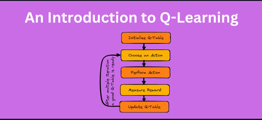
Q-table and How It Works

The Q-learning algorithm maintains a table (Q-table) where each entry corresponds to a state-action pair Q(s,a)Q(s, a)Q(s,a). Initially, the Q-table is populated with arbitrary values. As the agent interacts with the environment, it updates the Q-values using the Bellman equation:

Q(s, a) ← Q(s, a) + α [ R + γ * max_a’ Q(s’, a’) – Q(s, a) ]

Where:

• α\alphaα: The learning rate, which controls how much the new value overrides the old value.
• RRR: The reward received after taking action a from state s.
• γ\gammaγ: The discount factor, which determines the importance of future rewards. A value closer to 1 emphasizes long-term rewards, while a value closer to 0 focuses on immediate rewards.
• s′s’s′: The next state after action a is taken.
• max⁡a′Q(s′,a′)\max_{a’} Q(s’, a’)maxa′​Q(s′,a′): The maximum Q-value for the next state s’, indicating the best action the agent can take.

Algorithm Steps of Q-learning

1. Initialize the Q-table with arbitrary values for all state-action pairs.
2. Repeat the following steps until convergence:
   • Select an action aaa in the current state sss using an exploration strategy (e.g., ϵ\epsilonϵ-greedy).
   • Take the action and observe the reward RRR and the new state s′s’s′.
   • Update the Q-value for Q(s,a)Q(s, a)Q(s,a) using the Bellman equation.
   • Q(s, a) ← Q(s, a) + α [ R + γ * max_a’ Q(s’, a’) – Q(s, a) ]
   • Move to the new state s′s’s′.
3. End when a sufficient level of learning is reached, or after a fixed number of episodes.

Exploration vs. Exploitation

A crucial aspect of Q-learning is balancing exploration (trying new actions to discover their effects) and exploitation (choosing the best-known action to maximize rewards). This is often managed using an ϵ\epsilonϵ-greedy strategy, where the agent takes a random action with probability ϵ\epsilonϵ and chooses the action with the highest Q-value with probability 1−ϵ1 – \epsilon1−ϵ.

Strengths of Q-learning

• Model-free: Does not require a model of the environment, making it versatile and adaptable.
• Convergence: Proven to converge to the optimal policy under specific conditions (sufficient exploration and a decaying learning rate).
• Simplicity: Conceptually straightforward and easy to implement.

Limitations of Q-learning

• Scalability: The Q-table can become infeasibly large for environments with a large number of states, leading to high memory requirements.
• Continuous Action Spaces: Q-learning is not directly applicable to environments where actions are continuous.
• Sample Efficiency: Learning can be slow in complex environments where exploration requires many episodes.

Applications of Q-learning

Q-learning is applied in various domains, including:

• Game Playing: Training agents to play games like tic-tac-toe or simple video games.
• Robotics: Basic decision-making for simple robotic tasks.
• Navigation: Autonomous agents learning to navigate through grids or mazes.
• Resource Management: Optimal scheduling and resource allocation problems.

Example: Training an Agent to Navigate a Grid

Consider an agent navigating a 5×5 grid to reach a goal while avoiding obstacles:

• The agent starts with a Q-table initialized to zero.
• For each episode, it starts from a random position and takes actions (up, down, left, right) to maximize rewards.
• The reward structure could be:
  • +10 for reaching the goal.
  • -1 for each step taken.
  • -10 for hitting an obstacle.
• Over time, the agent learns the optimal path to the goal by updating its Q-table based on the Bellman equation.

Deep Q Networks (DQN): Bridging Q-learning and Deep Learning

Deep Q Networks (DQN) represent a significant advancement in the field of Reinforcement Learning (RL), combining the power of Q-learning with deep neural networks. Developed by DeepMind, DQNs made headlines for their success in training agents to play and excel at classic Atari games using raw pixel data. This approach addresses the limitations of traditional Q-learning in environments with large, continuous state spaces.

Why DQN?

Traditional Q-learning relies on a Q-table that stores Q-values for each state-action pair. This method works well for environments with discrete and small state spaces but fails when the state space becomes too large or continuous. In these scenarios, using a table to store Q-values is infeasible due to memory constraints and slow learning rates. DQN overcomes this limitation by using a deep neural network to approximate the Q-value function, allowing it to handle high-dimensional state spaces.

Key Components of DQN

1. Deep Neural Network: DQN uses a neural network as a function approximator to predict the Q-values for each action given a state. The input to the network is the current state, and the output is a vector of Q-values for all possible actions.
2. Experience Replay: This is a mechanism to improve the efficiency and stability of training. It works by storing past experiences (state, action, reward, next state) in a buffer called a replay memory. During training, random batches of experiences are sampled from the buffer to break the correlation between consecutive experiences and reduce the risk of overfitting.
3. Target Network: To further stabilize training, DQN maintains a separate target network that is used to generate the target Q-values. This network is a copy of the main Q-network but is updated less frequently. This approach helps prevent large, rapid changes in Q-values, making the training process more stable.

Algorithm Steps of DQN

Initialize the main Q-network and target Q-network with random weights

Q_network = initialize_network() # e.g., neural network
Q_target_network = initialize_network() # copy of Q_network

Initialize the replay memory to store experiences

replay_memory = ReplayMemory(capacity=10000)

Hyperparameters

gamma = 0.99 # Discount factor
epsilon = 0.1 # Exploration rate (for epsilon-greedy)
learning_rate = 0.00025
batch_size = 32 # Mini-batch size
update_target_freq = 1000 # Frequency of target network update

For each episode

for episode in range(total_episodes):
state = env.reset() # Reset environment, get initial state
done = False

while not done:
    # Choose action using epsilon-greedy policy
    if np.random.rand() < epsilon:
        action = np.random.choice(env.action_space)  # Random action (exploration)
    else:
        # Choose action with max Q-value from the current state using Q_network
        action = np.argmax(Q_network(state))  # Use the Q-network to predict best action

    # Take the action, observe reward, and next state
    next_state, reward, done, _ = env.step(action)

    # Store experience in the replay memory
    replay_memory.add(state, action, reward, next_state, done)

    # Sample a random mini-batch of experiences from the replay memory
    if len(replay_memory) >= batch_size:
        batch = replay_memory.sample(batch_size)
        states, actions, rewards, next_states, dones = zip(*batch)

        # Compute the target Q-value for each sampled experience
        targets = []
        for i in range(batch_size):
            if dones[i]:
                targets.append(rewards[i])  # If the episode is done, target = reward
            else:
                target = rewards[i] + gamma * np.max(Q_target_network(next_states[i]))  # Bellman equation
                targets.append(target)

        # Update the Q-network by minimizing the loss: L = (y - Q(s, a))^2
        Q_network.update(states, actions, targets, learning_rate)

    # Periodically copy weights from Q_network to Q_target_network
    if episode % update_target_freq == 0:
        Q_target_network.set_weights(Q_network.get_weights())

    # Move to the next state
    state = next_state

# Op

Explanation of the Code:

1. Initialization:
   • Q_network: The primary Q-network, typically a neural network that approximates the Q-value function.
   • Q_target_network: A separate target Q-network used for stable updates (it is periodically copied from the primary Q-network).
   • Replay memory: A data structure (e.g., a deque) that stores past experiences (state, action, reward, next state, done).
2. Exploration-Exploitation:
   • The agent uses an epsilon-greedy strategy to balance exploration (random actions) and exploitation (choosing actions based on Q-values).
3. Experience Replay:
   • The agent stores its experiences in the replay memory and samples random mini-batches to update the Q-network. This breaks the correlation between consecutive experiences, improving learning stability.
4. Q-value Update:
   • The target Q-value yyy is computed using the Bellman equation:pythonCopy codey = R + γ * max_a' Q_target(s', a') where RRR is the observed reward and max⁡a′Qtarget(s′,a′)\max_a’ Q_target(s’, a’)maxa′​Qt​arget(s′,a′) is the maximum Q-value for the next state using the target network.
   • The Q-network is then updated to minimize the loss:pythonCopy codeL = (y - Q(s, a))^2 where Q(s,a)Q(s, a)Q(s,a) is the predicted Q-value for the current state-action pair.
5. Target Network Update:
   • Periodically (every few episodes), the weights of the Q-network are copied to the target Q-network to stabilize learning.
6. Decay of Epsilon:
   • Epsilon decays over time to reduce exploration and favor exploitation as the agent learns.

Improvements in DQN

• Double DQN (DDQN): Addresses the overestimation bias in DQN by decoupling the selection of the action from the calculation of the target Q-value. This leads to more accurate value estimation.
• Dueling DQN: Splits the Q-network into two streams, one that estimates the value of being in a state and another that estimates the advantage of each action. This structure helps the network learn which states are valuable without having to learn the effect of each action for those states.
• Prioritized Experience Replay: Instead of sampling experiences uniformly from the replay buffer, experiences that are more significant (with higher TD errors) are sampled more frequently. This prioritization allows the agent to focus on learning from the most informative experiences.

Advantages of DQN

• Handles Complex State Spaces: DQN can learn directly from high-dimensional inputs, such as images, which is not feasible with traditional Q-learning.
• Stable Training: The use of experience replay and a target network helps stabilize the training process, reducing oscillations and divergence.

Applications of DQN

1. Atari Game Playing: DQN was famously used by DeepMind to train agents that surpassed human-level performance in many Atari 2600 games by learning directly from pixel data and game scores.
2. Robotics: DQN can be applied to train robots in simulated environments where they learn tasks like object manipulation and navigation.
3. Autonomous Driving: DQN has been used in research for training agents to handle specific tasks in simulated driving environments, such as lane-keeping and obstacle avoidance.

Challenges with DQN

• Sample Inefficiency: DQN often requires a large number of interactions with the environment to learn effectively, making training time-consuming.
• Instability in Training: Despite experience replay and target networks, training can sometimes be unstable, particularly in environments with sparse rewards.
• Continuous Action Spaces: DQN, in its basic form, is not suitable for continuous action spaces, as it outputs discrete Q-values for each possible action.

Policy Gradient Methods: An Overview

Policy Gradient Methods are a class of algorithms in Reinforcement Learning (RL) that directly optimize the policy (i.e., the mapping from states to actions) by following the gradient of expected rewards. Unlike value-based methods like Q-learning and Deep Q Networks (DQN), which focus on learning value functions and deriving policies from them, policy gradient methods aim to learn the policy itself.

Why Policy Gradient Methods?

Policy gradient methods are particularly useful in environments where:

• Continuous Action Spaces: Value-based methods struggle with continuous actions, whereas policy gradients can naturally handle these.
• Stochastic Policies: In scenarios where randomness is beneficial (e.g., exploration in dynamic environments), policy gradients can directly learn stochastic policies, unlike deterministic policies derived from value functions.
• Flexible Policy Representation: The policy can be parameterized using any function approximator, such as neural networks, allowing for more complex and adaptable policies.

Mathematics Behind Policy Gradients

The goal of policy gradient methods is to maximize the expected return J(θ)J(\theta)J(θ), where θ\thetaθ represents the parameters of the policy. The expected return is defined as:

J(θ)=Eπθ[∑t=0TRt]J(\theta) = \mathbb{E}_{\pi_{\theta}} \left[ \sum_{t=0}^{T} R_t \right]J(θ)=Eπθ​​[∑t=0T​Rt​]

The core idea is to adjust the policy parameters θ\thetaθ in the direction that increases J(θ)J(\theta)J(θ). This adjustment is achieved using the policy gradient theorem, which provides an unbiased estimator for the gradient:

∇θJ(θ)=Eπθ[∇θlog⁡πθ(at∣st)R(τ)]\nabla_{\theta} J(\theta) = \mathbb{E}_{\pi_{\theta}} \left[ \nabla_{\theta} \log \pi_{\theta}(a_t | s_t) R(\tau) \right]∇θ​J(θ)=Eπθ​​[∇θ​logπθ​(at​∣st​)R(τ)]

Where:

• πθ(at∣st)\pi_{\theta}(a_t | s_t)πθ​(at​∣st​) is the probability of taking action ata_tat​ in state sts_tst​ under the policy parameterized by θ\thetaθ.
• R(τ)R(\tau)R(τ) is the total reward obtained for a trajectory τ\tauτ.

REINFORCE Algorithm

The REINFORCE algorithm is one of the simplest policy gradient methods. It uses Monte Carlo sampling to estimate the gradient and update the policy parameters:

1. Collect Trajectories: Run the current policy in the environment and collect trajectories (state, action, reward).
2. Compute Returns: Calculate the cumulative return for each trajectory.
3. Update Parameters: Use the gradient update rule: θ←θ+α∑t=0T∇θlog⁡πθ(at∣st)R(τ)\theta \leftarrow \theta + \alpha \sum_{t=0}^{T} \nabla_{\theta} \log \pi_{\theta}(a_t | s_t) R(\tau)θ←θ+α∑t=0T​∇θ​logπθ​(at​∣st​)R(τ) Where α\alphaα is the learning rate.
4. Initialize policy network with random weights
   policy_network = initialize_policy_network()
   Hyperparameters
   learning_rate = 0.01
   gamma = 0.99 # Discount factor
   For each episode
   for episode in range(total_episodes):
   state = env.reset()
   done = False
   trajectory = [] # To store (state, action, reward) tuples for the episode
   while not done: action = choose_action(state, policy_network) # Select action from policy next_state, reward, done, _ = env.step(action) # Store the experience trajectory.append((state, action, reward)) # Move to next state state = next_state # Calculate the cumulative returns for each step in the episode returns = calculate_returns(trajectory, gamma) # Update the policy parameters using the REINFORCE rule for t in range(len(trajectory)): state, action, reward = trajectory[t] return_ = returns[t] grad_log_policy = compute_gradient_log_policy(state, action, policy_network) policy_network.update(grad_log_policy * return_, learning_rate)

Advantages:

• Simple to implement.
• Effective in problems with small to moderate complexity.

Limitations:

• High variance in gradient estimates, which can lead to unstable learning.
• Requires complete episodes to calculate rewards, which can be inefficient.

Actor-Critic Methods

To address the high variance issue in the REINFORCE algorithm, Actor-Critic methods were developed. These methods combine the benefits of policy gradients (actor) and value-based methods (critic) to create a more stable learning process.

• Actor: Represents the policy πθ\pi_{\theta}πθ​, which decides the actions.
• Critic: Estimates the value function V(s)V(s)V(s) or the advantage function A(s,a)A(s, a)A(s,a) to critique the actions taken by the actor.

Assume we have a policy network (actor) and a value network (critic)

Initialize the policy and value networks with random weights

policy_network = initialize_policy_network() # Actor network
value_network = initialize_value_network() # Critic network

Hyperparameters

learning_rate_actor = 0.01 # Learning rate for actor (policy network)
learning_rate_critic = 0.01 # Learning rate for critic (value network)
gamma = 0.99 # Discount factor

For each episode

for episode in range(total_episodes):
state = env.reset() # Reset environment for each new episode
done = False
trajectory = [] # Store (state, action, reward, value) tuples

while not done:
    # Select action based on policy network (actor)
    action = choose_action(state, policy_network)  # Using the policy network

    # Execute action in environment and get the next state, reward, and done flag
    next_state, reward, done, _ = env.step(action)

    # Estimate value for current state using the critic (value network)
    value = value_network(state)

    # Store the experience tuple (state, action, reward, value) in trajectory
    trajectory.append((state, action, reward, value))

    # Move to the next state
    state = next_state

# Compute cumulative returns (target values) for each time step in the trajectory
returns = calculate_returns(trajectory, gamma)

# Compute advantages for each time step
advantages = calculate_advantages(trajectory, value_network)  # Advantage function A(s_t, a_t)

# Update critic (value network) and actor (policy network)
for t in range(len(trajectory)):
    state, action, reward, value = trajectory[t]
    advantage = advantages[t]  # A(s_t, a_t)

    # Update critic (value network) using Temporal Difference (TD) error
    td_error = reward + gamma * value_network(next_state) - value
    value_network.update(td_error, learning_rate_critic)  # Update critic

    # Update actor (policy network) using the policy gradient with advantage scaling
    grad_log_policy = compute_gradient_log_policy(state, action, policy_network)  # ∇θ log π_θ(a_t | s_t)
    policy_network.update(grad_log_policy * advantage, learning_rate_actor)  # Update actor with advantage scaling

Policy Gradient Algorithms

1. REINFORCE: The simplest form of policy gradient algorithm, using complete returns for gradient updates.
2. Actor-Critic: Combines policy gradient (actor) and value function approximation (critic) for more stable learning.
3. Proximal Policy Optimization (PPO): A popular and more stable policy gradient method that uses a clipped surrogate objective to prevent large policy updates, improving training stability and performance.
4. Trust Region Policy Optimization (TRPO): Enforces a constraint on the step size during policy updates to maintain stability, although it can be computationally expensive.

Advantages of Policy Gradient Methods

• Direct Policy Optimization: Enables learning of stochastic and continuous policies directly.
• Handles Continuous Spaces: Can naturally handle continuous action spaces without discretization.
• Adaptability: Policies can be flexible and adapt to dynamic environments.

Challenges and Limitations

• High Variance: Gradient estimates can have high variance, leading to slow or unstable learning.
• Sample Inefficiency: Policy gradient methods may require a large number of interactions with the environment to learn effectively.
• Sensitivity to Hyperparameters: Performance can be sensitive to the choice of learning rate and other hyperparameters.

Applications of Policy Gradient Methods

1. Robotics: Teaching robots to perform tasks involving fine motor control, such as grasping objects or walking.
2. Game Playing: Training agents to play games like Go, chess, and complex real-time strategy games. Policy gradient methods were a component in DeepMind’s AlphaGo.
3. Autonomous Vehicles: Enabling self-driving systems to learn policies for driving safely in various conditions and environments.
4. Finance: Learning trading strategies in algorithmic trading.

conclusion

Reinforcement Learning (RL) has rapidly evolved, bringing powerful tools and methods to solve complex decision-making problems across various domains. Q-learning, Deep Q Networks (DQN), and Policy Gradient Methods represent three critical advancements that have shaped the landscape of RL.

Q-learning laid the groundwork as a simple, yet effective algorithm for learning optimal policies in discrete environments without needing prior knowledge. Its straightforward update rule enabled RL agents to learn from trial and error by mapping states to actions and adjusting policies based on rewards. However, Q-learning’s limitations, such as scalability issues with large state spaces, called for further innovations.

Deep Q Networks (DQN) emerged as a significant milestone that extended Q-learning’s capabilities to environments with high-dimensional state spaces. By leveraging deep neural networks, DQN approximated Q-values and enabled agents to learn complex tasks directly from raw sensory data, such as pixels. This advancement, popularized by DeepMind’s success in training agents to achieve superhuman performance in Atari games, demonstrated the potential of combining deep learning with RL.

Policy Gradient Methods provided another leap by directly optimizing policies, making them ideal for handling continuous action spaces and learning stochastic policies. Unlike value-based methods that derive policies from value functions, policy gradients learn the policy itself, allowing for more flexible decision-making strategies. The emergence of Actor-Critic methods and further developments like Proximal Policy Optimization (PPO) enhanced the stability and efficiency of policy gradient training.

Applications Across Industries

These algorithms have found applications in various fields:

• Robotics: RL algorithms like DQN and policy gradient methods are used to teach robots complex tasks such as navigation, object manipulation, and interaction with dynamic environments. The adaptability and continuous learning capability of policy gradient methods are particularly valuable in these applications.
• Game Playing: The use of RL in game playing reached new heights with AlphaGo, which combined policy gradient methods with Monte Carlo Tree Search and neural networks to defeat human champions in the game of Go. This showcased RL’s ability to master strategic decision-making in competitive and high-dimensional spaces.
• Autonomous Vehicles: RL is applied in training self-driving vehicles to handle real-world driving scenarios, from basic lane-keeping to advanced decision-making in complex traffic situations. The ability of DQN and policy gradients to learn from simulations and adapt in real-time makes them crucial for the development of safe and efficient autonomous systems.

Final Thoughts

The journey from Q-learning to DQN and Policy Gradient Methods represents the evolution of RL from basic, discrete task-solving to mastering high-dimensional, continuous environments with adaptable policies. Each method contributes unique strengths, shaping the way intelligent agents learn and interact with their surroundings. As RL continues to advance, its impact will expand, driving innovations in robotics, gaming, autonomous vehicles, and beyond, ultimately moving us closer to creating intelligent systems capable of autonomous decision-making and complex problem-solving in real-world scenarios.