A Comprehensive Guide to key machine Learning Aligorithms 2024

http://A Comprehensive Guide to key machine Learning Aligorithms 2024

Machine learning (ML) is at the forefront of modern artificial intelligence (AI) and is widely used across industries to solve complex problems. In this blog post, we will explore some of the most fundamental machine learning algorithms, their key concepts, mathematical foundations, and Python code implementations.

We will focus on the following key algorithms:

1. Linear Regression
2. Logistic regression
3. Decision Trees
4. Random Forests
5. Support Vector Machines (SVM)
6. k-Nearest Neighbors (k-NN)
7. Gradient Boosting (XGBoost, LightGBM, CatBoost)

Let’s dive in and explore each one in detail.

1. Linear Regression

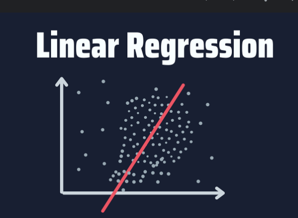
Linear regression is one of the simplest and most commonly used algorithms for regression tasks (predicting continuous values). The goal is to find a relationship between the independent variable XXX and the dependent variable YYY by fitting a linear equation.

Type: Supervised Learning
Use Case: Predictive analysis (e.g., housing prices, sales forecasting)
Description: Linear regression models the relationship between a dependent variable and one or more independent variables by fitting a linear equation. The goal is to find the best-fitting line that minimizes the error between predicted and actual values.

Formula:

The linear regression model is represented as:Y=β0+β1X+ϵY = \beta_0 + \beta_1X + \epsilonY=β0​+β1​X+ϵ

Where:

• YYY is the predicted value.
• XXX is the input feature.
• β0\beta_0β0​ is the intercept (bias term).
• β1\beta_1β1​ is the slope (weight).
• ϵ\epsilonϵ is the error term.

Python Implementation:

pythonCopy codefrom sklearn.linear_model import LinearRegression

# Sample data
X = [[1], [2], [3], [4], [5]]  # Feature values
y = [1, 2, 3, 4, 5]  # Target values

# Create the model and fit it to the data
model = LinearRegression()
model.fit(X, y)

# Predicted value for X = 6
prediction = model.predict([[6]])
print(f"Predicted Value: {prediction[0]}")

2. Logistic regression

Logistic regression is used for classification tasks where the goal is to predict a categorical label (e.g., binary classes). It models the probability that a given input belongs to a particular class.

Type: Supervised Learning (Classification)
Use Case: Binary classification (e.g., spam detection, customer churn prediction)
Description: Logistic regression estimates the probability that an instance belongs to a particular class by fitting data to a logistic function. It’s used for binary and multiclass classification.

Formula:

The logistic regression model uses the sigmoid function:P(y=1∣X)=11+e−(β0+β1X)P(y = 1|X) = \frac{1}{1 + e^{-(\beta_0 + \beta_1X)}}P(y=1∣X)=1+e−(β0​+β1​X)1​

Where:

• P(y=1∣X)P(y = 1|X)P(y=1∣X) is the probability of the positive class.
• XXX is the input feature.
• β0\beta_0β0​ and β1\beta_1β1​ are the parameters to be learned.

Python Implementation:

pythonCopy codefrom sklearn.linear_model import LogisticRegression

# Sample data for binary classification
X = [[1], [2], [3], [4], [5]]
y = [0, 0, 1, 1, 1]  # Binary target labels

# Create and fit the logistic regression model
model = LogisticRegression()
model.fit(X, y)

# Predict probability for X = 6
prediction = model.predict_proba([[6]])[0][1]
print(f"Predicted Probability of Class 1: {prediction}")

3. Decision Trees

Decision Trees are versatile models used for both regression and classification tasks. The model splits the data into subsets based on feature values, creating a tree-like structure. The algorithm recursively chooses the feature that best separates the data at each level.

Type: Supervised Learning
Use Case: Customer segmentation, decision analysis
Description: Decision trees split the dataset into branches to make decisions based on feature conditions. Each node represents a feature, each branch a decision, and leaves indicate the outcome. They are interpretable and handle both numerical and categorical data.

Formula:

The decision tree algorithm does not have a fixed formula but uses concepts like Gini impurity or Entropy to make decisions.

• Gini Impurity for a node ttt is defined as:

G(t)=1−∑i=1Cpi2G(t) = 1 – \sum_{i=1}^{C} p_i^2G(t)=1−i=1∑C​pi2​

Where pip_ipi​ is the proportion of class iii in the node.

• Entropy is another criterion:

Entropy(t)=−∑i=1Cpilog⁡2(pi)Entropy(t) = – \sum_{i=1}^{C} p_i \log_2(p_i)Entropy(t)=−i=1∑C​pi​log2​(pi​)

Where pip_ipi​ is the proportion of class iii in the node.

Python Implementation:

pythonCopy codefrom sklearn.tree import DecisionTreeClassifier

# Sample data for classification
X = [[1], [2], [3], [4], [5]]
y = [0, 0, 1, 1, 1]

# Create and train the Decision Tree classifier
model = DecisionTreeClassifier()
model.fit(X, y)

# Predict for X = 6
prediction = model.predict([[6]])
print(f"Predicted Class: {prediction[0]}")

4. Random Forests

Random Forest is an ensemble learning method based on decision trees. It creates multiple decision trees and combines their outputs to make predictions. Each tree is trained on a random subset of the data with bootstrapping (sampling with replacement).

Type: Supervised Learning (Ensemble Method)
Use Case: Fraud detection, recommendation systems
Description: A random forest is an ensemble of decision trees that operate by training multiple trees and aggregating their outputs for improved accuracy and robustness. It reduces the risk of overfitting seen in single decision trees.

Formula:

Random Forests do not have a single formula, but their logic is an extension of decision trees. The final prediction is the average (for regression) or the majority vote (for classification) of the individual trees.

Python Implementation:

pythonCopy codefrom sklearn.ensemble import RandomForestClassifier

# Sample data for classification
X = [[1], [2], [3], [4], [5]]
y = [0, 0, 1, 1, 1]

# Create and train the Random Forest model
model = RandomForestClassifier(n_estimators=100)
model.fit(X, y)

# Predict for X = 6
prediction = model.predict([[6]])
print(f"Predicted Class: {prediction[0]}")

5. Support Vector Machines (SVM)

Support Vector Machines are powerful classifiers that work by finding the hyperplane that best separates the classes in a high-dimensional space. The key idea is to maximize the margin between the classes

Type: Supervised Learning
Use Case: Text classification, image recognition
Description: SVMs work by finding the hyperplane that best separates the data into classes. They are effective in high-dimensional spaces and are suitable for both linear and non-linear classification using the kernel trick.

Formula:

SVM aims to solve the following optimization problem:min⁡w,b12∣∣w∣∣2\min_{\mathbf{w}, b} \frac{1}{2} ||\mathbf{w}||^2w,bmin​21​∣∣w∣∣2

Subject to the constraints:yi(w⋅xi+b)≥1,∀iy_i (\mathbf{w} \cdot \mathbf{x}_i + b) \geq 1, \quad \forall iyi​(w⋅xi​+b)≥1,∀i

Where:

• w\mathbf{w}w is the weight vector.
• bbb is the bias term.
• yiy_iyi​ is the label of the i-th sample.

Python Implementation:

pythonCopy codefrom sklearn.svm import SVC

# Sample data for classification
X = [[1], [2], [3], [4], [5]]
y = [0, 0, 1, 1, 1]

# Create and train the SVM model
model = SVC(kernel='linear')
model.fit(X, y)

# Predict for X = 6
prediction = model.predict([[6]])
print(f"Predicted Class: {prediction[0]}")

6. k-Nearest Neighbors (k-NN)

k-Nearest Neighbors is a simple and intuitive algorithm for classification and regression. It classifies new data points based on the majority class of their k nearest neighbors in the training dataset.

Type: Supervised Learning
Use Case: Recommender systems, pattern recognition
Description: KNN is a non-parametric algorithm used for both classification and regression. It classifies a data point based on the majority class among its k-nearest neighbors. It’s simple and effective for smaller datasets.

Formula:

The prediction is based on the majority class (for classification) or the average of the target values (for regression) of the k-nearest neighbors.

Python Implementation:

pythonCopy codefrom sklearn.neighbors import KNeighborsClassifier

# Sample data for classification
X = [[1], [2], [3], [4], [5]]
y = [0, 0, 1, 1, 1]

# Create and train the k-NN model
model = KNeighborsClassifier(n_neighbors=3)
model.fit(X, y)

# Predict for X = 6
prediction = model.predict([[6]])
print(f"Predicted Class: {prediction[0]}")

7. Gradient Boosting (XGBoost, LightGBM, CatBoost)

Gradient Boosting is an ensemble technique that builds models sequentially, with each new model correcting the errors made by the previous ones. XGBoost, LightGBM, and CatBoost are highly optimized libraries for gradient boosting that offer better performance and scalability.

Type: Supervised Learning (Ensemble Method)
Use Case: Competition-winning algorithms, predictive modeling
Description: Gradient boosting algorithms build trees sequentially, each one correcting the errors of the previous tree. Variants like XGBoost, LightGBM, and CatBoost provide optimizations for handling large datasets efficiently.

Formula (General Gradient Boosting):

In gradient boosting, the new model is fitted on the residuals (errors) of the previous model:Fm(x)=Fm−1(x)+η⋅hm(x)F_m(x) = F_{m-1}(x) + \eta \cdot h_m(x)Fm​(x)=Fm−1​(x)+η⋅hm​(x)

Where:

• Fm(x)F_m(x)Fm​(x) is the prediction after the mmm-th model.
• hm(x)h_m(x)hm​(x) is the weak model (e.g., decision tree) at the mmm-th step.
• η\etaη is the learning rate.

Python Implementation (XGBoost):

pythonCopy codeimport xgboost as xgb
from sklearn.datasets import load_breast_cancer
from sklearn.model_selection import train_test_split

# Load dataset
data = load_breast_cancer()
X = data.data
y = data.target

# Split the data
X_train, X_test, y_train, y_test = train_test_split(X, y, test_size=0.3, random_state=42)

# Create and train the XGBoost model
model = xgb.XGBClassifier()
model.fit(X_train, y_train)

# Predict and evaluate
prediction = model.predict(X_test)
print(f"Predicted Class: {prediction[0]}")